Introduction
The p-value is a continuous measure of statistical evidence, yet in practice it is often reduced to a binary decision: p < 0.05 is “significant”, p ≥ 0.05 is “not significant”. This dichotomous thinking contributes to the reproducibility crisis in science.
The p3d package visualizes the p-value of a single-sample t-test as a three-dimensional surface over two parameters:
- Effect size (d, Cohen’s d)
- Sample size (n)
This vignette demonstrates the core functionality of the package.
The p-value surface
The central function of the package is p_surface().
Given a range of effect sizes and sample sizes, it computes the p-value
for each combination:
surface <- p_surface(
  d = seq(-2, 2, 0.1),
  n = seq(5, 200, 5)
)

str(surface, max.level = 1)
#> List of 6
#>  $ d     : num [1:41] -2 -1.9 -1.8 -1.7 -1.6 -1.5 -1.4 -1.3 -1.2 -1.1 ...
#>  $ n     : num [1:40] 5 10 15 20 25 30 35 40 45 50 ...
#>  $ p     : num [1:41, 1:40] 0.0111 0.0132 0.0158 0.0191 0.0232 ...
#>  $ d_crit: num [1:40] 1.242 0.715 0.554 0.468 0.413 ...
#>  $ alpha : num 0.05
#>  $ grid  :'data.frame':  1640 obs. of  5 variables:
#>   ..- attr(*, "out.attrs")=List of 2
The result is a list with several components:
-
d: the vector of effect sizes -
n: the vector of sample sizes -
p: a matrix of p-values (dimensionslength(d)×length(n)) -
d_crit: critical effect sizes at α = 0.05 for each n -
alpha: the significance level -
grid: a tidy data frame with all combinations
Inspecting the results
For example, the p-value at d = 0.5, n = 30 is:
surface$p[surface$d == 0.5, surface$n == 30]
#> [1] 0.01043739
The critical effect size at n = 30 is:
surface$d_crit[surface$n == 30]
#> [1] 0.3734061
This means: with 30 observations, an effect size of at least 0.37 is required for statistical significance at α = 0.05.
Static 3D visualization
The simplest way to visualize the surface is
plot_p_static(), which uses base R graphics and has
no external dependencies:
plot_p_static(surface)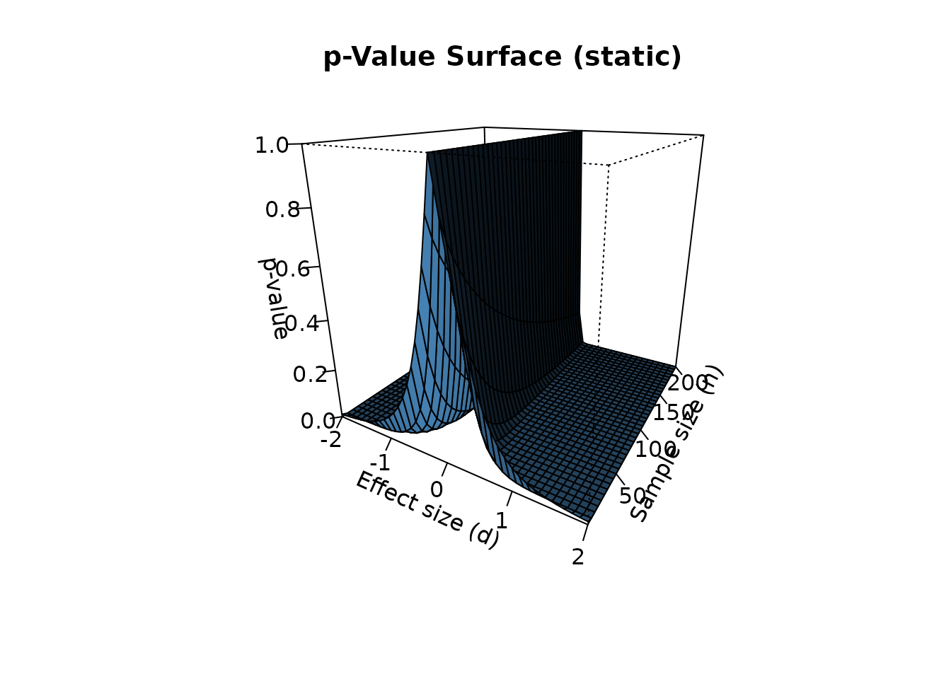
This is ideal for PDF output, journal figures, and printed reports.
Interactive 3D visualization
For interactive exploration, use plot_p_surface() with
the plotly engine:
plot_p_surface(surface, engine = "plotly")Alternatively, the rgl engine provides a native R
window:
plot_p_surface(surface, engine = "rgl")Both engines allow rotation, zooming, and panning.
2D comparison
For comparison with existing 2D packages such as
pvaluefunctions, use p_curve_2d():
curve_30 <- p_curve_2d(d = seq(-2, 2, 0.1), n = 30)
head(curve_30)
#>      d            p significant
#> 1 -2.0 8.021139e-12        TRUE
#> 2 -1.9 2.650857e-11        TRUE
#> 3 -1.8 9.099432e-11        TRUE
#> 4 -1.7 3.247269e-10        TRUE
#> 5 -1.6 1.205427e-09        TRUE
#> 6 -1.5 4.654771e-09        TRUE
The 2D curve is mathematically equivalent to a slice of the 3D surface at fixed n.
Real-data example
Let’s apply p3d to a real dataset. The
mtcars dataset contains fuel consumption (mpg) for 32
automobiles. Suppose we want to test whether the mean mpg is different
from 20:
x <- mtcars$mpg
d_obs <- (mean(x) - 20) / sd(x)
n_obs <- length(x)

cat("Observed effect size:", round(d_obs, 4), "\n")
#> Observed effect size: 0.015
cat("Sample size:", n_obs, "\n")
#> Sample size: 32
The p-value for this single observation is:
By placing this observation on the 3D surface, we can see how the same effect size would behave at different sample sizes:
surface_real <- p_surface(
  d = seq(-0.5, 0.5, 0.01),
  n = seq(5, 200, 5)
)

plot_p_static(surface_real, theta = 30, phi = 20)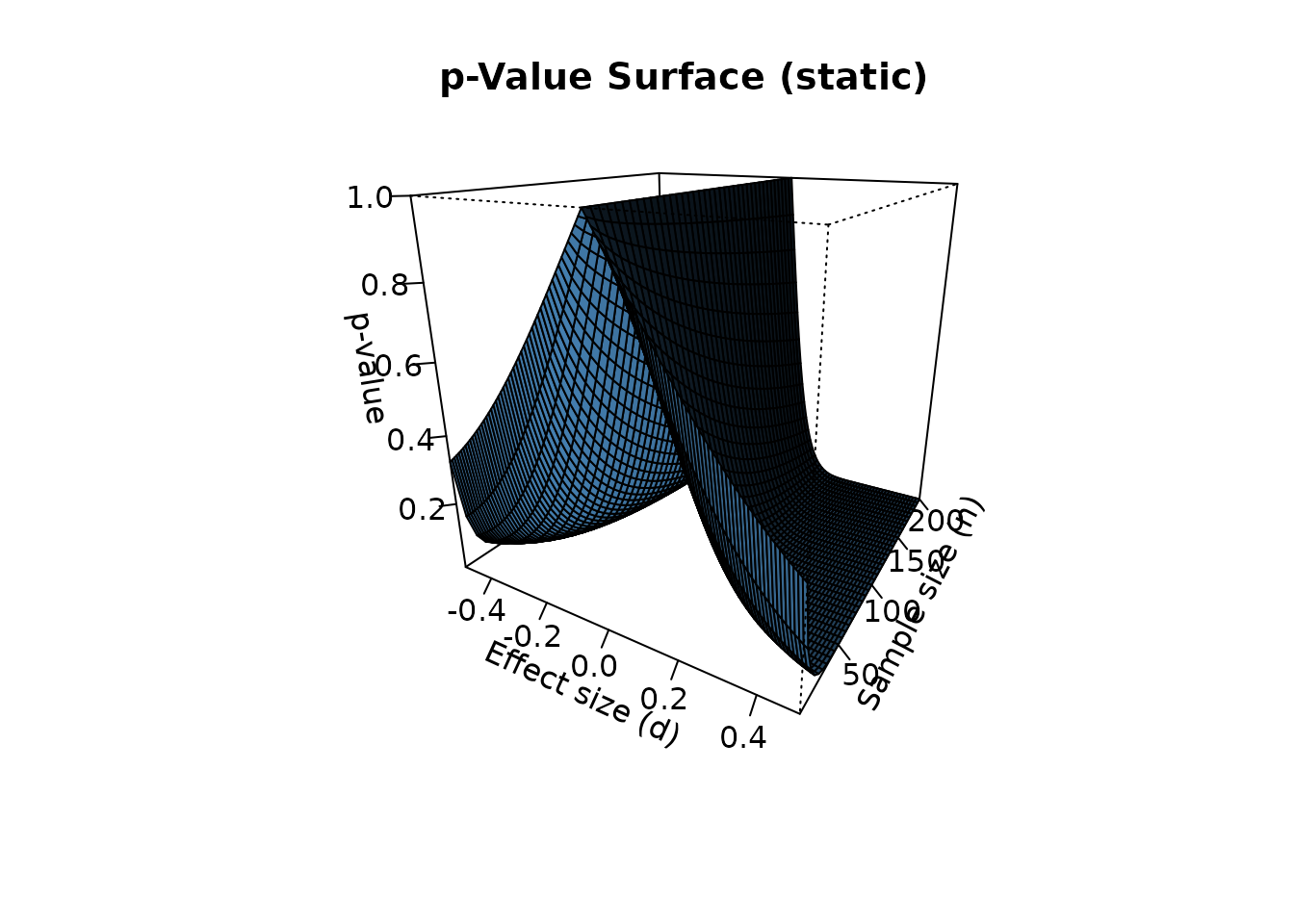
Conclusion
The p3d package provides a three-dimensional perspective on the p-value. By visualizing the p-value simultaneously across effect size and sample size, it reveals:
- The continuous nature of the p-value (it is not a binary switch)
- The moderating effect of sample size on statistical significance
- The interaction between effect size and sample size
This complements traditional 2D visualizations and helps weaken the dichotomous thinking that plagues statistical practice.
References
Helske, J., Helske, S., Cooper, M., Ynnerman, A., & Besançon, L. (2021). Can Visualization Alleviate Dichotomous Thinking? Effects of Visual Representations on the Cliff Effect. IEEE Transactions on Visualization and Computer Graphics, 27(8), 3496-3509.
Cohen, J. (1988). Statistical Power Analysis for the Behavioral Sciences (2nd ed.). Lawrence Erlbaum Associates.