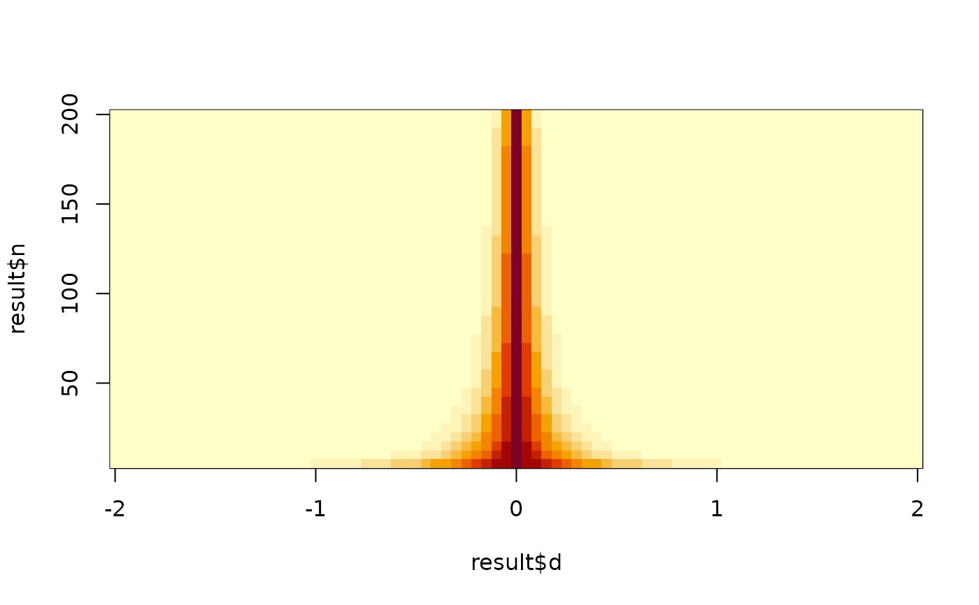
Computes the p-value of a single-sample t-test as a function of effect size (Cohen's d) and sample size (n). Returns a grid of p-values suitable for 3D visualization.
Value
A list with the following elements:
- d
The input vector of effect sizes.
- n
The input vector of sample sizes.
- p
A matrix of p-values with dimensions
length(d)xlength(n).- d_crit
A numeric vector of critical effect sizes for each sample size at level
alpha.- alpha
The significance level used.
- grid
A data frame with the full grid of (d, n, p) combinations.
Details
The p-value is computed using the formula: $$p(d, n) = 2 \left[ 1 - F_{t(n-1)}(d \sqrt{n}) \right]$$ where \(F_{t(n-1)}\) is the cumulative distribution function of the t-distribution with \(n-1\) degrees of freedom.
The critical effect size at level \(\alpha\) is: $$d_{crit}(n) = \frac{F^{-1}_{t(n-1)}(1 - \alpha/2)}{\sqrt{n}}$$
Examples
# Small example
result <- p_surface(d = seq(-1, 1, 0.1), n = c(10, 30, 100))
str(result)
#> List of 6
#>  $ d     : num [1:21] -1 -0.9 -0.8 -0.7 -0.6 -0.5 -0.4 -0.3 -0.2 -0.1 ...
#>  $ n     : num [1:3] 10 30 100
#>  $ p     : num [1:21, 1:3] 0.0115 0.0192 0.0322 0.0541 0.0903 ...
#>  $ d_crit: num [1:3] 0.715 0.373 0.198
#>  $ alpha : num 0.05
#>  $ grid  :'data.frame':	63 obs. of  5 variables:
#>   ..$ d     : num [1:63] -1 -0.9 -0.8 -0.7 -0.6 -0.5 -0.4 -0.3 -0.2 -0.1 ...
#>   ..$ n     : num [1:63] 10 10 10 10 10 10 10 10 10 10 ...
#>   ..$ t_stat: num [1:63] -3.16 -2.85 -2.53 -2.21 -1.9 ...
#>   ..$ df    : num [1:63] 9 9 9 9 9 9 9 9 9 9 ...
#>   ..$ p     : num [1:63] 0.0115 0.0192 0.0322 0.0541 0.0903 ...
#>   ..- attr(*, "out.attrs")=List of 2
#>   .. ..$ dim     : Named int [1:2] 21 3
#>   .. .. ..- attr(*, "names")= chr [1:2] "d" "n"
#>   .. ..$ dimnames:List of 2
#>   .. .. ..$ d: chr [1:21] "d=-1.0" "d=-0.9" "d=-0.8" "d=-0.7" ...
#>   .. .. ..$ n: chr [1:3] "n= 10" "n= 30" "n=100"

# Typical use
result <- p_surface(d = seq(-2, 2, 0.05), n = seq(5, 200, 5))
image(result$d, result$n, result$p)